 Forge SPC GuidesForge SPC
X̄-R chart walkthrough: a machining process
Goal
A 5-axis machining center turns an outside diameter to 73.99 mm (LSL 73.88, USL 74.10). Five parts are measured every sampling period, 25 times. You want to know two things:
- Is the process stable? — are there signs of special causes over those 25 periods?
- Is it capable? — does its spread fit inside the tolerance?
This guide answers both with the example project Forge SPC installs on first run. Every number below is what the app shows for that project.
The data
- Characteristic: outside diameter (mm)
- Subgroups: 25 × n = 5 (125 readings)
- Specification: LSL 73.88 · Target 73.99 · USL 74.10
- Story behind it: a stable start, then tool wear drifts the mean upward, then the tool is replaced
The data is synthetic and was built to behave like a real tool-wear episode, so the signals you will see are there on purpose.
Step 1 — Open the example project
On first run the home screen already holds X-bar R Machining Process. Open it.
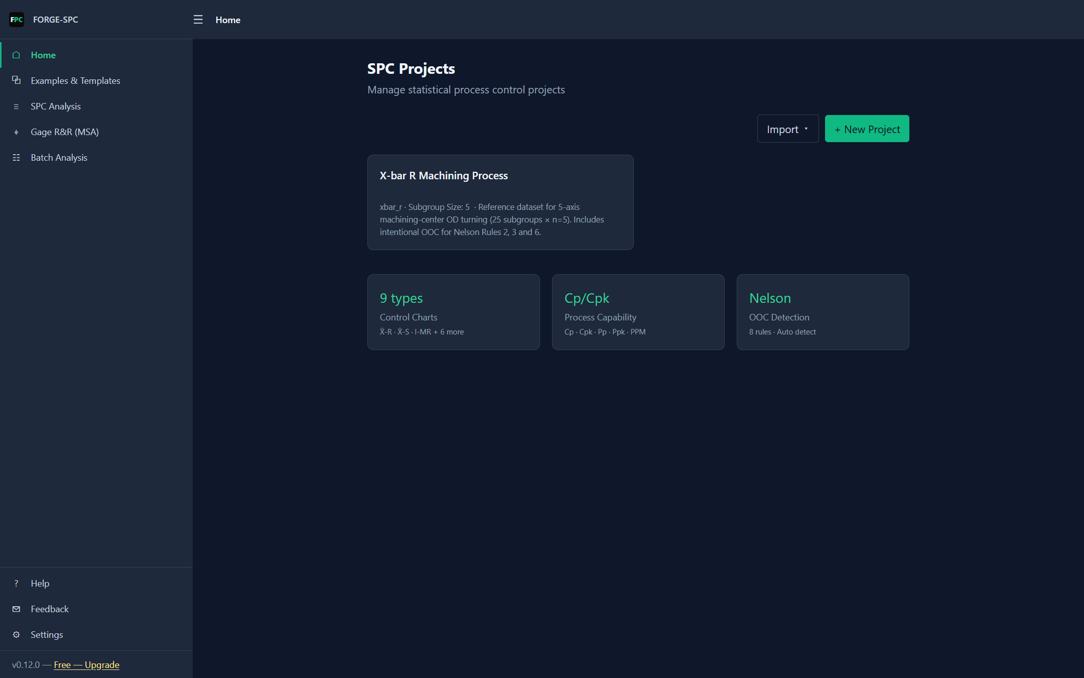
You can add it again at any time from Examples & Templates.
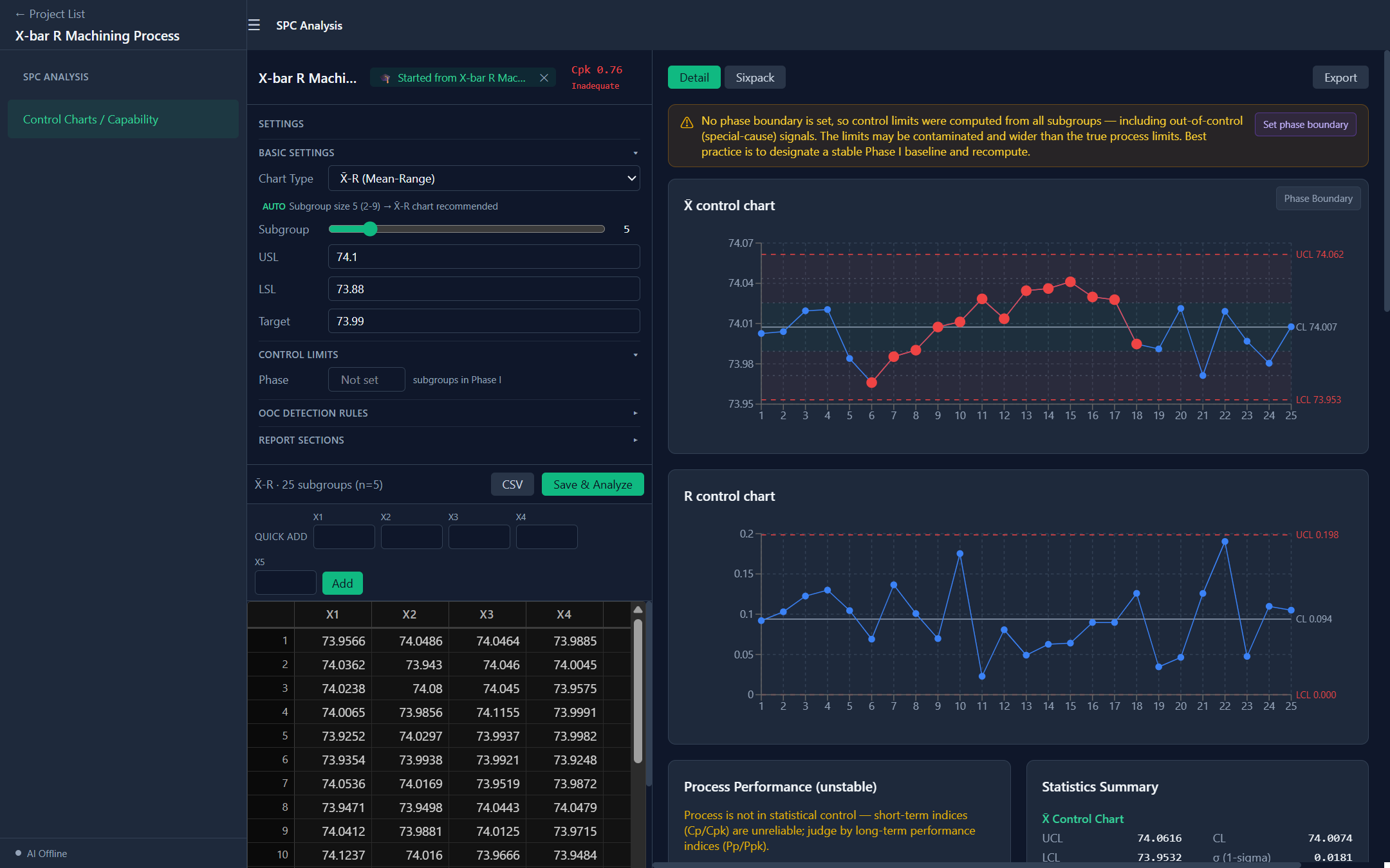
The chart page has three parts: settings and data on the left, charts and analysis on the right, and Export at the top right.
Step 2 — Check the chart type and the specification
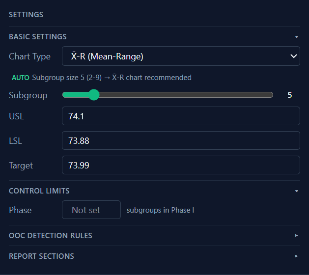
- Chart type: X̄-R. Forge recommends it from the subgroup size (marked AUTO): X̄-R for 2 to 9 readings per subgroup, X̄-S above that, where the standard deviation makes fuller use of each subgroup than the range does.
- USL / LSL / Target are the drawing's tolerance. They do not affect the control limits — only the capability indices.
Step 3 — Notice that the limits are contaminated
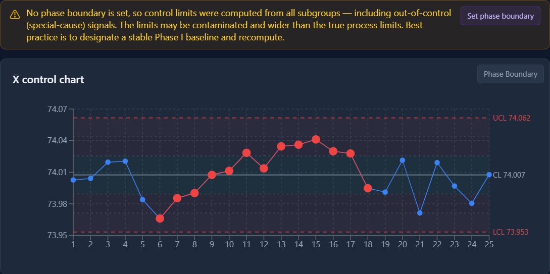
With no boundary set, Forge computes the limits from all 25 subgroups — X̄: UCL 74.062, CL 74.007, LCL 73.953; R: UCL 0.198, CL 0.094 — and says so in the banner above the chart.
That matters because control limits are supposed to describe the process when only common causes are acting. Subgroups 9–17 were made while the tool was wearing; averaging them into the center line moves it toward the drift, and the chart ends up judging the drift against a reference that already contains it.
The red points are subgroups that take part in a rule violation. Note that none of them is beyond the limits — the signals here are patterns, not single outliers.
Step 4 — Set a Phase I baseline
Phase I is the stretch of data you accept as the reference; Phase II is everything judged against it. In the settings panel, under Control Limits → Phase, enter 8. (Or press Set phase boundary and click subgroup 8 on the chart.)
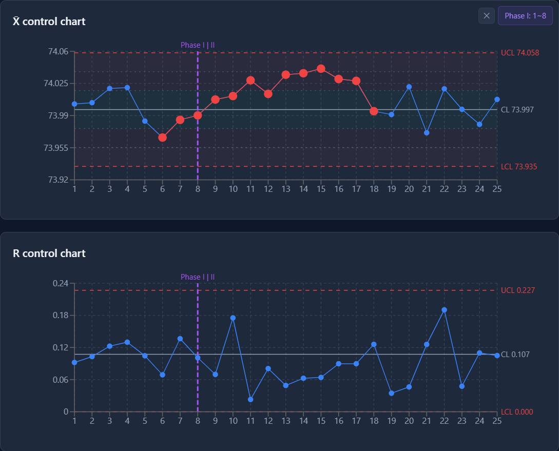
The charts now draw a Phase I | II line after subgroup 8 and show Phase I: 1~8. The limits are recomputed from the baseline only:
| All 25 subgroups | Phase I = 1–8 | |
|---|---|---|
| X̄ UCL / CL / LCL | 74.062 / 74.007 / 73.953 | 74.058 / 73.997 / 73.935 |
| R UCL / CL | 0.198 / 0.094 | 0.227 / 0.107 |
Two things worth seeing here:
- The center line moved down, back to where the process was before the drift (73.997).
- The limits did not get narrower. The first eight subgroups happen to have slightly larger ranges, so the R chart's limits widened. A baseline is chosen because it is free of special causes, not because it produces tighter limits.
Why 8? The template's story puts the start of tool wear at subgroup 9. In a real study the boundary comes from your own records — a tool change, a new material lot, a setup. Eight subgroups is a short baseline; treat limits from it as provisional and recompute once more in-control data has accumulated.
Step 5 — Read the signals
Scroll to Signal Diagnosis.
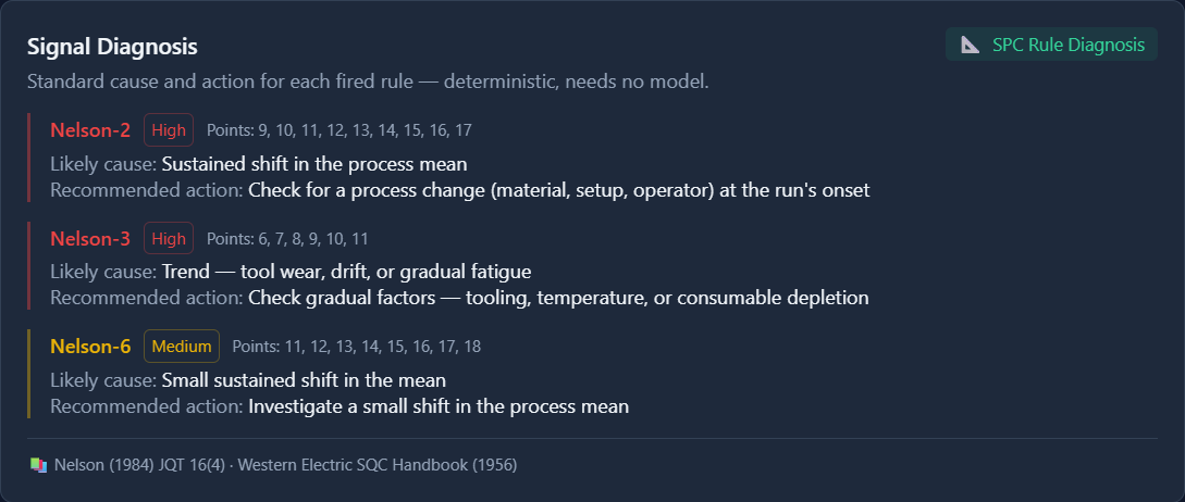
Each rule that fired is listed with the subgroups involved, a likely cause and a recommended action:
| Rule | Subgroups | What it says |
|---|---|---|
| Nelson 2 — 9 points in a row on one side of the center line | 9–17 | The mean has shifted and stayed there |
| Nelson 3 — 6 points in a row steadily increasing or decreasing | 6–11 | A trend: wear, drift, temperature |
| Nelson 6 — 4 of 5 points beyond 1σ on the same side | 11–18 | A smaller but sustained shift |
Read them together: a rising run (rule 3) turns into a sustained high level (rules 2 and 6), then ends at subgroup 18 — the tool-wear-then-replacement pattern.
The trend signal covers subgroups 6–11 as a run. It does not by itself mean subgroups 6–8 were already out of control, which is why the baseline in step 4 can still end at 8 — but it is exactly the kind of evidence you should check against the process log before accepting a baseline.
The OOC Signals count in the statistics summary is 23. It counts rule violations, not points: a subgroup that takes part in two rules is counted twice.
These causes and actions are fixed, rule-by-rule text — no AI is involved. If the local AI model is installed, AI Root Cause Analysis below can draft a cause hypothesis from the same signals.
Step 6 — Judge capability
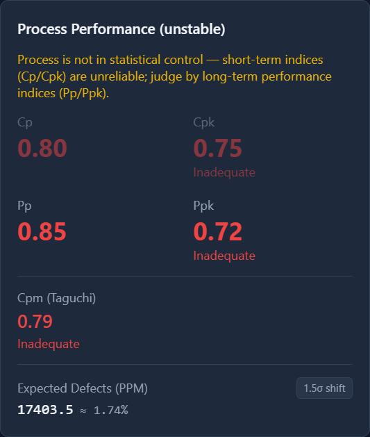
Because the process is not in statistical control, the card is titled Process Performance (unstable) and dims Cp and Cpk:
- Cp / Cpk (0.80 / 0.75) use the within-subgroup spread (R̄ / d₂ from the Phase I baseline). They predict what the process could do if it stayed stable — a prediction you cannot rely on while signals are present.
- Pp / Ppk (0.85 / 0.72) use the overall spread of all 125 readings. They describe what the process did do, drift included. For an unstable process these are the honest numbers.
Ppk 0.72 is below 1 — the process mean sits closer to the USL than the spread allows. Expected Defects — 17,403.5 PPM ≈ 1.74 % — is the share of a normal distribution with the overall mean and spread that falls outside the tolerance. The 1.5σ shift button switches it to the six-sigma convention, which assumes the mean will drift by a further 1.5σ in the long term.
"Stable" and "capable" are separate questions. Even once the tool wear is controlled, the within-subgroup capability (Cp 0.80) is short of 1: the spread itself is too wide for this tolerance.
Step 7 — Check the normality assumption

Capability indices and the expected-defect figure read the spread against a normal distribution — a 3σ distance means 0.135 % beyond it only if the data is roughly normal. The Anderson-Darling test here gives A² = 0.3695, p = 0.4266 — no evidence against normality (p > 0.10), so the indices can be read as they are. When the test rejects normality, Forge offers non-normal capability methods instead.
Step 8 — Export the result
Export at the top right opens the export options.
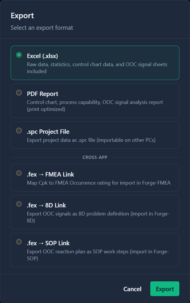
- PDF Report — charts, capability and signal analysis for sharing.
- Excel (.xlsx) — raw data, statistics, chart data and signals, one sheet each.
- .fex → FMEA / 8D / SOP — hand the result to the other Forge apps: the capability as an FMEA occurrence rating, the signals as an 8D problem description, or the reaction plan as SOP steps.
What to take away
- Limits computed over a period that contains special causes describe the wrong process. Set a Phase I baseline from your process records.
- Rule signals are patterns — a run, a trend — as often as they are single points beyond the limits.
- While the process is unstable, judge capability by Pp/Ppk; Cp/Cpk say what it could achieve once stable.
- Stability and capability are separate problems with separate remedies.
References
- Montgomery, D. C. Introduction to Statistical Quality Control, 8th ed. Wiley, 2019, ch. 6.
- ISO 7870-2:2023 (Shewhart control charts).
- AIAG. Statistical Process Control (SPC) Reference Manual, 2nd ed., 2005.
- Nelson, L. S. Journal of Quality Technology 16(4), 1984, pp. 237–239.
- Anderson, T. W., and Darling, D. A. Journal of the American Statistical Association 49(268), 1954.