When a p chart flags half the days: overdispersion and Laney's p′ chart
With large subgroups, a p chart's binomial limits get so narrow that ordinary day-to-day variation lands outside them. What overdispersion is, how Laney's p′ chart measures it with σz, a worked example where the p chart flags 10 of 20 days and the p′ chart flags one, and what σz below 1 means.
On this page
A p chart plots the fraction defective of each subgroup against limits that come from the binomial distribution. With a few hundred parts per subgroup it works as intended. With tens of thousands of parts per subgroup it often stops working: half the points fall outside the limits, nothing special happened on those days, and people learn to ignore the chart.
David Laney described this in Quality Engineering in 2002 and proposed a fix, the p′ chart (read "p prime"). This article shows where the problem comes from, what the p′ chart changes, and how to read its one extra number, σz.
Where the binomial limits come from
For a subgroup of nᵢ parts and an average fraction defective p̄, the p chart's limits are
UCLᵢ, LCLᵢ = p̄ ± 3 · σₚᵢ, σₚᵢ = √( p̄(1 − p̄) / nᵢ )
σₚᵢ is the spread you would expect from sampling alone, if every subgroup came from a process with exactly the same true fraction defective p̄. It shrinks with √n. At p̄ = 2 % and n = 23,000, three σₚᵢ is about 0.28 percentage points: any day outside 1.73 %–2.29 % is a signal.
But a real process does not keep exactly the same true rate from day to day. Material lots, shifts, setups and the weather move it a little. That day-to-day movement does not shrink with n. In Laney's words, p charts "assume that all the variation in the entire process is within-subgroup variation, or sampling variation" — and when the samples are large, "the P chart puts the control limits too close together and the data seem to be escaping."
When the subgroup-to-subgroup variation is larger than the binomial formula predicts, the data are overdispersed.
What the p′ chart changes
Laney's chart keeps the binomial limits' shape (each subgroup still gets its own width from its own nᵢ) and multiplies them by one factor measured from the data:
- Standardize each point: zᵢ = (pᵢ − p̄) / σₚᵢ. If the binomial model were the whole story, the zᵢ would have a standard deviation of 1.
- Measure how much they actually vary, with the moving range of consecutive points: σz = MR̄ / 1.128, where MR̄ is the average of |zᵢ − zᵢ₋₁| and 1.128 is the d₂ constant for ranges of two.
- Widen (or narrow) the limits by that factor: UCLᵢ, LCLᵢ = p̄ ± 3 · σₚᵢ · σz.
σz is "the relative amount of process variation not explained by the binomial assumption alone", as SPC for Excel's write-up of the method puts it. σz = 1 gives back the ordinary p chart. σz = 3 says the subgroups vary three times as much as sampling alone explains.
The moving range is the same estimator an individuals (I-MR) chart uses, so the p′ chart treats the subgroups like a sequence of individual measurements, while still letting a large subgroup have narrower limits than a small one.
A worked example: 10 signals become one
Twenty days of final inspection on a high-volume line, between 20,000 and 30,000 parts a day. The data are synthetic: each day's true rate varies around 2 % with a standard deviation of 0.22 percentage points, and on day 15 the true rate was raised to 3.2 % — one real special cause.
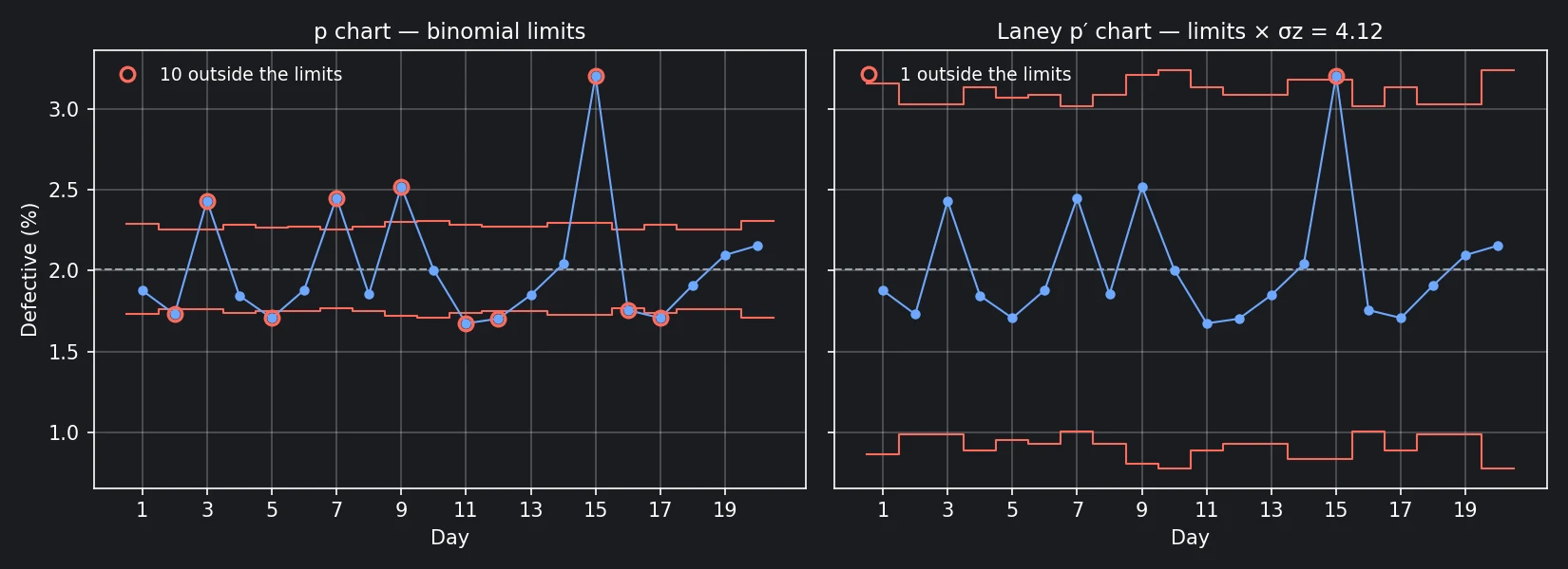
- p chart (binomial limits): 10 of the 20 days are outside the limits — days 2, 3, 5, 7, 9, 11, 12, 15, 16 and 17. Nine of the ten are ordinary day-to-day variation.
- p′ chart: σz = 4.12. The limits are 4.12 times wider, and only day 15 is outside — at 3.20 % against an upper limit of 3.18 %.
Day 15 barely clears its limit, and part of the reason is day 15 itself. The two moving ranges on either side of it are the largest in the series (12.3 and 15.8). Leave those two out and σz would be 3.15, not 4.12. A large special cause inflates the σz that the limits are built from, so the p′ chart is conservative about the very point that inflated it. Once a cause is found and removed, the limits for the next period should come from data without it.
The data, so you can reproduce the numbers (n = parts inspected, d = defectives):
| Day | n | d | Day | n | d | |
|---|---|---|---|---|---|---|
| 1 | 23,000 | 432 | 11 | 24,000 | 402 | |
| 2 | 29,000 | 502 | 12 | 26,000 | 443 | |
| 3 | 29,000 | 705 | 13 | 26,000 | 481 | |
| 4 | 24,000 | 443 | 14 | 22,000 | 449 | |
| 5 | 27,000 | 461 | 15 | 22,000 | 705 | |
| 6 | 26,000 | 489 | 16 | 30,000 | 527 | |
| 7 | 30,000 | 735 | 17 | 24,000 | 410 | |
| 8 | 26,000 | 482 | 18 | 29,000 | 554 | |
| 9 | 21,000 | 529 | 19 | 29,000 | 608 | |
| 10 | 20,000 | 401 | 20 | 20,000 | 431 |
In total, 10,189 defectives in 507,000 parts: p̄ = 2.010 %.
σz below 1
σz can also come out below 1: the subgroups vary less than sampling alone would explain. The p′ chart then narrows the limits, and a point can signal on the p′ chart that would not on the ordinary p chart.
Underdispersion is not a sign of an unusually steady process. Binomial sampling sets a floor on how much a fraction defective varies between random samples, and data that vary less than that floor usually did not come from random samples — stratified sampling (each subgroup deliberately mixes the same sources in the same proportions) and autocorrelated data (consecutive subgroups sharing parts or material) are the usual reasons. Check how the subgroups were drawn before treating a signal on a narrowed chart as a process change.
When to use it
Laney's own answer, asked whether there are conditions where the p′ chart should not be used, was "No. Categorically, positively, no." His reasoning is that σz ≈ 1 gives the same limits as the p chart, so nothing is lost when the binomial model holds: "Even if Sigma Z is 1.01, I'd still rather use the P' chart!"
Two practical limits:
- σz is estimated from moving ranges, so it needs a sequence in time order, and with very few subgroups it is a rough estimate.
- The p′ chart corrects the limits. It does not explain the extra variation. A σz of 4 is itself a finding: something moves the defect rate from day to day by much more than sampling does, and finding out what may be worth more than the chart.
Try it in Forge SPC
In Forge SPC, a p chart with three or more subgroups is drawn as a Laney p′ chart. The chart carries a Laney P′ badge with the measured σz, and the stats table, the PDF report and the Excel export print the same limits and the same σz, so the limits a point is judged on are the limits every page states. When σz is below 1, the chart page, the report and the Excel sheet say that the limits were narrowed and that the samples may not be random.
Two bundled projects show both directions: P-Chart PCB SMT Defect Rate (Laney P′) is overdispersed (σz ≈ 2.25, from a systematic difference between the morning and afternoon shifts), and the plating defect example is underdispersed (σz ≈ 0.53).
References
- D. B. Laney, "Improved control charts for attributes", Quality Engineering, 14(4), 2002, pp. 531–537, doi:10.1081/QEN-120003555.
- Minitab Blog Editor, "On the Charts: A Conversation with David Laney", Minitab Blog, 4 October 2011.
- SPC for Excel, "Laney p' Control Chart" (knowledge base article).
- ISO 7870-2:2023, Control charts — Part 2: Shewhart control charts — the p chart with limits for each subgroup size.